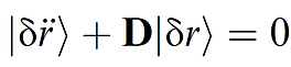


(1a)
(2)
(3)
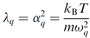
(4)
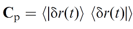
(5)
(6)
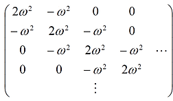
D =
(1b)
A perfect 1D mono-atomic solid with N atoms can be represented as a 1D spring, with nearest neighbor interactions.
The only difference is that initial conditions are specified by equipartition, such that all modes carry equal kT amount of energy.
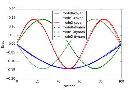
One can verify that the covariance matrix (Cp) eigenvalues and eigen vectors converges to the dynamical matrix (D) eigen vectors, and that eigen values of covariance matrix = 1/evals of dynamical matrix. The caveat is that the ordering is opposite: low-frequency modes correspond to large eigenvalues of Cp, and small eigenvals of D.
In this tutorial, I verify that indeed the covariance matrix converges to that which is expected, from the dynamical matrix . (Big help from Henkes et. al Soft Matter, 2011)
STEP 1: Choose appropriate frequency omega (w) for the dynamical matrix (In Eqn. 1a, b). To make matters simple, I chose w=1, kT=1, mass m=1. Then, diagonalize D to find eigenvals of D (Eqn. 2). I chose fixed edge boundary conditions for 100 atoms (0th and 99th not moving), connected by springs.
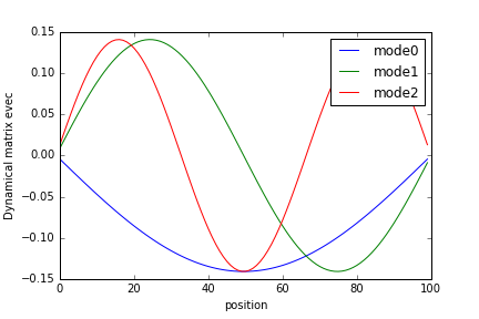
The eigenvectors are shown below, corresponding to the 3 lowest frequencies, i.e. 3 lowest Eigenvals.
PRO TIP: Eigenvectors and eigenvals are not always sorted, so make sure to sort Evecs corresponding to sorted evals before plotting!
STEP 2: Initialize the spring system through equipartition initial conditions (Eqn. 3, 4). This is a critical step, and for me the most confusing. It's simple enough, just to follow Eqn. 3. However keep in mind, you need to sum over all modes, i.e. for the displacement of the 'ith' atom at t=0, we need to sum over all modes (all q's) corresponding to position 'i'.
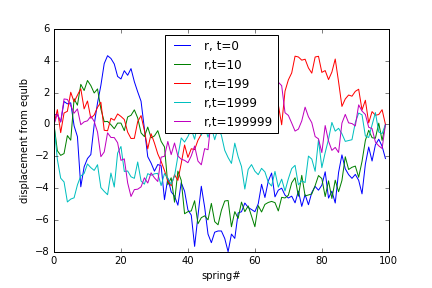
STEP 3: Now that we know the initial conditions, we can plug back into Eqn. 1a, b and numerically solve for dynamics! Below is a graph showing the time evolution of spring displacements over time, as well as a gif of first 20 atoms.
PRO tip: Simple Euler method to numerically solve, almost definitely gives numerical error leading to growing perturbations, which are unrealistic. To ensure numerical stability, I used the Verlet algorithm, of course there are multiple methods you can use, such as Runge-Kutta.
STEP 4: Now that we have the displacement magnitidues, we can compute Cp (Eqn. 5). In Eqn. 5, 't' corresponds to a picked time interval, during which displacement is measured (r(t+t0)-t(t)), averaged over many t0. Similar to dynamical matrix, Cp can be diagonalized to find eigen values and eigen vectors, and thus verify Eqn. 6.
PRO TIP: Make sure that number of time intervals>2*Np/1.5, where Np is number of atoms (here 100), and choose time interval appropriately. Make sure time interval is large enough - atleast ~50 times natural time scale. For more details on convergence of empirically measure covariance matrix to the true correlation matrix, see Henkes et al. Soft Matter 2011.
In a similar eigen vector plot, you can see that the empirically measure eigenvectors from Cp, fall right on top of the eigen vectors from D! Albeit a phase shift for the 3rd mode, which is OK. Note: lowest frequency modes correspond to the smallest eigenvals of D, but the largest eigenvals of Cp. Also, from Eqn. 4, in reduced units, Evals of Cp should be=1/(Evals of D), and the figures shown below show that this is indeed the case! The noise is due to empirically measured Cp. Thus, I verified that the evals and evecs from measured Cp are consistent with actual Dynamical matrix. Thus this is a robust method that can potentially be used to find harmonic interactions in empirical systems.